How Does a Meteorological Model Work ?
Accuracy and Resolution
Dr. John W. (Jack) Glendening, Meteorologist
Updated: Dec 31, 2007
This webpage gives a basic description of how meteorological models
generate their predictions, with an emphasis on model errors and the
influence of model resolution. It is intended to provide a
framework for discussions of weather prediction models and their
errors. Additional information on errors of particular
importance to BLIPMAP predictions is given in the Model Notes
webpage.
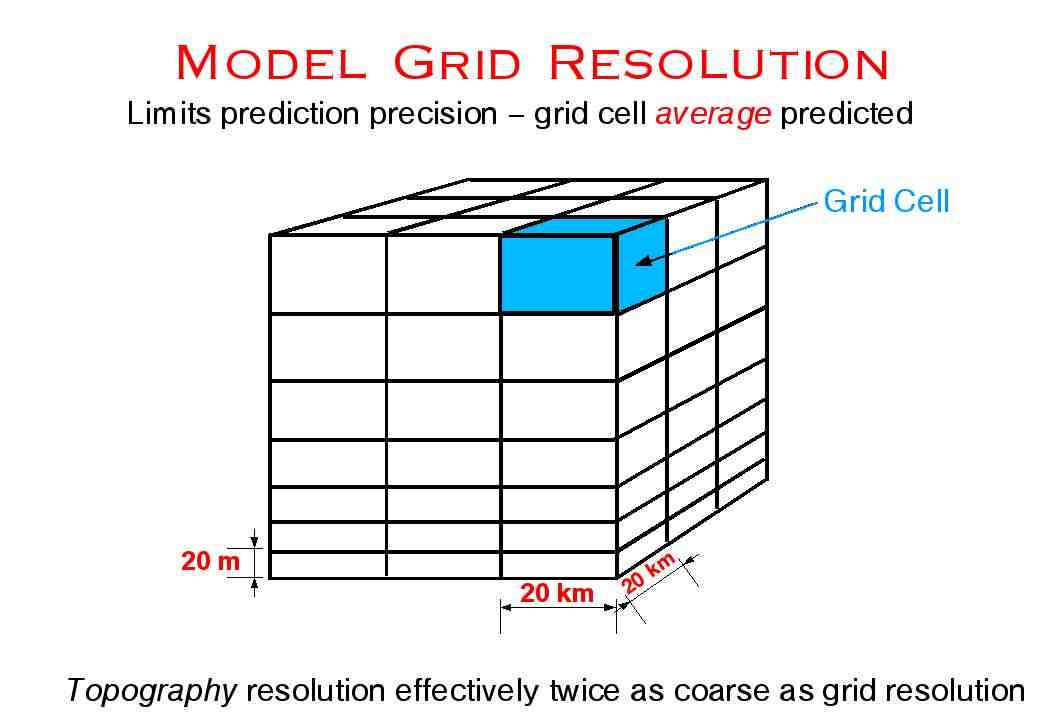
The Grid
Numerical meteorological models produce predictions by solving
equations at grid points created by dividing the atmosphere into cells
and forecasting the average of each predicted variable over that
cell. Generally cells are regularly spaced in the
horizontal but vary in the vertical, with vertical spacings becoming
smaller near the surface since atmospheric conditions change more rapidly with
height there. Similarly, vertical cell spacings in general are
much smaller than horizontal spacings since conditions
change much more rapidly in the vertical than in the horizontal. (See the Grid
Cell Diagram)
The Equations of Motion
A meterological model produces forecasts by solving the "equations of
motion" for a fluid, which are derived from fundamental physical laws:
conservation of mass (both of air and moisture), conservation of
momentum (Newton's laws), and conservation of thermal energy
(thermodynamics). These equations predict the change in
variables such as temperature or velocity resulting from the physical
phenomena which affect them. These equations strongly interact with
each other - for example, a change in thermal energy (affecting
temperature) will change atmospheric density (affecting mass), in turn
changing pressure differences (affecting velocity). These feedback
interactions tend to counter a forced change, e.g. to oppose an
atmospheric heating by introducing a cooling effect. If forcing were
to remain constant then eventually the feedbacks would produce an
"equilibrium" in which changes with time would become increasingly
smaller - but the forcing of the atmosphere is never constant, as
solar heating is constantly changing, so the atmosphere is in a state
of constantly adjusting "quasi-equilibrium".
Solution Methodology
What is being solved is a set of "Partial Differential Equations",
where the PDEs predict the time-change of a variable based upon
conditions in each central cell and its horizontal/vertical
neighbors. Those who have taken calculus will remember that
differential equations only apply to "infinitesimally" small spacings
so we are assuming that a "finite difference" over the finite grid
spacing is a reasonable approximation to a differential. The
equations are solved in a "marching-forward-in-time" fashion, starting
from the assumed 3D initial conditions (which are usually based on
available observations at that time), and predicting how the
variables change at each time step at each grid point to give
forecasts at a given time. PDEs are solved for the
"prognostic variables" of temperature, humidity, the three components
of velocity, condensed moisture (clouds), etc. The model also
calculates "diagnostic" variables which depend solely upon conditions
at the present time (so they depend upon the prognostic variables but
do not have to be solved in a "time-marching" fashion).
Since all the equations are inter-related, an error in any one will to
some degree affect the others. These PDEs are not
empirical equations, since they are fundamentally derived from
well-established physical laws of conservation of energy and momentum
and mass.
Model Initialization
Since the equations of motion predict changes there must be an
initially prescribed 3D atmosphere for them to start from. This is
obtained from atmospheric observations (baloon, satellite, and
aircraft data) at a limited number of points which are then
interpolated to complete the 3D grid. There will of course be errors
in the interpolated initial state (it is not a solution of the
equations of motion), so initially the equations predict relatively
large changes as they evolve towards the equation of motion
quasi-equilibrium. Forecasts during this "spinup" period are subject
to large errors and should be taken with a grain of salt, since they
reflect the initial "interpolated" guess. Spinup inaccuracies
decrease with time - within the BL, the minimum-to-maximum spinup time
is roughly 1-to-4 hours, the longer time being for larger grid
spacings and larger initial errors (spinup times are longer
above the BL).
Overall Prediction Accuracy
Forecast accuracy of the many parameters predicted by a
meteorological model can be generally ordered, from most accurate to
least accurate, as: (1) Winds, (2) Thermal
parameters, (3) Moisture parameters, (4) Cloud
parameters, (5) Rainfall.
Model Errors
The accuracy of the a model depends on many factors, which can be
roughly grouped as:
-
Time Step Errors:
Since the equations represent the change over an "infinitesimal" time
but the actual time step is finite, errors will occur with larger time
steps creating larger errors. The actual time step used is, like
much else in numerical modeling, a compromise between the ideal and
the practical.
-
Initial Condition Errors:
The model requires "Initial Conditions" to start from, needing
"knowledge" of the full three-dimensional atmosphere i.e. all
prognostic variables at every grid point! This is obtained by
combining available observations - notably, but not limited
to, observed soundings - with previous model predictions to
produce an initial "analysis". This analysis must be done
carefully while respecting the dynamic constraints of the equations,
i.e. is not a matter of simple interpolation of observations, since a
large error introduced between observing points would cause large and
unrealistic changes immediately after startup as the equations tried
to adjust to an unrealistic initial imbalance. Correct initial
conditions can be important to model predictions, but are less important
at later times and closer to the surface. Initial conditions are
most important for predicting the progress of disturbances above the
BL, such as frontal movement.
-
Lateral Boundary Condition Errors:
A 20 km resolution model cannot cover the entire world, so such a
"fine-mesh" model is "nested" inside a "coarse-mesh" model, having
larger-spacing and larger domain, which provides "neighboring" cells along
the lateral (outside) boundary of the fine-mesh model. The
coarse-grid model typically covers the entire globe (though sometimes
there will be multiple "nestings" to get to the global model).
Errors in the lateral boundary conditions will, over time, reach
further into the fine-mesh grid so lateral BC errors can be reduced by
increasing the size of the fine-mesh domain - but of course
that takes additional grid points and computational time and given
finite constraints on each the choice of a lateral boundary is always
a trade off. The model domain used by the RAP model can be viewed
here.
By comparison, the NAM grid is much larger, reaching from the North
Pole to the Equator!
-
Surface Boundary Condition Errors:
The model must know the type of surface the atmosphere is interacting
with since its roughness, vegetation type, soil type and water
content, etc. all affect model predictions. This is the one true
boundary the atmosphere has and creates the "Boundary Layer" (BL) so
of course the predicted BL is especially affected by surface boundary
errors! A major difficulty is that "average" conditions for all
of surface quantities must be known for each of the surface model grid
cells while in reality these quantities vary over much smaller scales
so trying to, first, know what the actual surface consists of and,
secondly, create a meaningful average for each grid cell are both
subject to much error. Additionally, certain variables such as
vegetation and soil moisture vary with time. Further, trying to
predict soil moisture in detail would require calculations as
intensive as that for the atmosphere itself, so greatly simplified
equations are used instead.
-
Inadequate Spatial Resolution Errors:
The use of differential equations assumes/requires that a feature is
"resolved" by the grid resolution. If the effect of a lake or
mountain ridge or whatever upon the atmosphere is to be predicted, the
model must adequately "know" about the existence of that lake or ridge
or whatever. Realistic resolution requires a minimum of
four grid points inside such a feature. Modelers keep trying,
within the bounds of available computer power, to use finer and finer
grid resolutions since with present grid spacings there is still much
that is not being resolved, particularly if the forcing is controlled
by topography. There are also many atmospheric
features such as convergence-created upward motions which are
smaller than can be resolved with present model grids and so are not
well predicted. This error can be thought of as error that
occurs because the PDE equations assume changes over an
infinitesimally small distance whereas the model can only
estimate changes over a finite distance - if in
reality changes occurs over a smaller distance than the grid can
effectively resolve, the finite-difference equations then cannnot
accurately represent the actual differences existing in the
atmosphere.
-
Model "Noise" Errors:
One result of the limited resolution resulting from use of a
finite-spacing grid is that model "noise" develops, particularly at
the smallest resolveable scales. Physically this is because
energy in the atmosphere tends to be generated at relatively large
scales and then break down into successively smaller eddies. The
"differential" PDEs can and do simulate this behavior but only when
resolution of atmospheric eddies is adequate, which is not true when
the eddy size becomes comparable to the grid spacing - so in
the model energy breaks down until it reaches the smallest model scale
(i.e. the smallest resolvable eddy size)
and is then trapped there. As a result, model predictions often
vary at the smallest model scale in a saw-tooth manner, e.g. a
forecast variable will be too large at one cell, then too small at the
neighboring cell, and then again too large at the next cell,
etc. This is typically reduced by "numerical filtering", but too
much filtering also throws away part of the true signal so a
compromise is required (as is typical in numerical
modeling!). Often one can see evidence of this model noise not
being fully controlled when a "bullseye" pattern appears in a BLIPMAP,
with the value at one grid point being much larger/smaller than its
surrounding neighbors. Decreasing model grid spacing helps to
reduce model noise, but it will always exist to some degree.
-
Model Topography Errors:
Generally model conditions represent "average" conditions over the
extent of its grid cell, but the effect of surface elevation on the
model is somewhat different since the topography used by a model is
typically smoothed to a coarser resolution than that of the
model grid spacing and can differ significantly from the actual
topography, particularly when the actual surface elevation changes
abruptly. The reason for this degradation is the model noise
problem discussed above: if the topography were to be fully
resolved then much noise would be generated at the very smallest
scale, aggravating the normal model noise build-up problem at that scale, so to
avoid this the very smallest scales are filtered out of the
topography. Note that this means that 8 model points are now
required to resolve a ridge, so resolution of surface elevation
influences requires a finer grid spacing than for many other atmospheric
influences.
Another terrain factor is that models often use an "envelope
topography" to produce better velocity predictions - but that can
result in worsened BL predictions, such as for BL top. The idea
behind an "envelope topography" is that in reality velocities on
either side of a mountain ridge, the Sierras being a good example, are
separated by a relatively high ridge; but if one uses elevations
averaged over 20 km (or larger!) cells then the ridge largely
disappears, so flows at a level which are not interacting in reality
will be interacting in the model. Therefore a weighting
is employed which pushs model topography toward the higher elevations
that actually exist over each grid cell rather than to a simple
average. However, other parameters such as surface temperature
and the BL driven by it do depend upon the average elevation over
a grid cell, so use of an envelope topography makes those predictions
less accurate! Sometimes a compromise solution is
attempted - for example, the RAP model has two
topographies, a "normal" (envelope) topography used for most
calculations and a "minimum" topography used for surface temperature
adjustments.
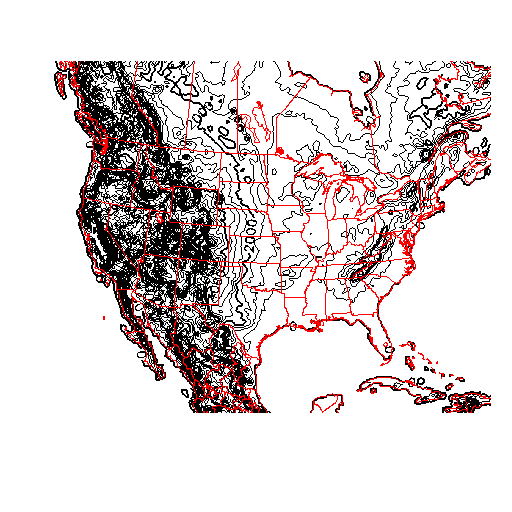
Additional discussion of differences between the smoothed model topography and
the real topography, with two illustrations, can be found on the
Grid Orientation webpage.
-
Parameterization Errors:
"Parameterization" refers to model terms which cannot be obtained from
fundamental principles so instead are computed from approximated
equations. For example, a model which has a 20 km resolution
cannot resolve many small clouds, yet those clouds affect the
atmosphere through effects such as release of heat aloft in
condensation, reduction of solar radiation reaching the surface,
etc. Since these effects are important but can't be predicted
explicitly by model equations/resolution, they must be
"parameterized". Parametrization is the "voodoo" part of
numerical modeling since it tries to predict complex processes using
necessarily over-simplified assumptions. Many cloud forecast
terms fall into this category.
[In one sense this might be described as an "inadequate resolution"
error, but here the resolution increase required to obtain
fundamnetally correct equations is so large that it cannot be achieved
in the foreseeable future, if ever, so is a unique problem. An
example familiar to soaring pilots is the formation of small puffy
cumulus clouds - these start out is small wisps of visible
vapor and even the cell resolution needed to resolve such wisps is
well beyond anything presently possible but to predict this
truly correctly one would have to resolve down to the cloud
droplet scale! A non-cloud example which is theoretically
more do-able but still impossible in practice is predicting the upward
transfer of heat in the BL - in reality this occurs though eddies such
as thermals and downdrafts which would need to be resolved, but that
would take a grid spacing of less than 50 m so instead it is
parameterized as a grid-average vertical transfer.]
-
End User Errors:
I cannot resist adding this after noting that some users misuse the
predictions by incorrectly applying the model-produced forecasts,
apparently due to a lack of appropriate knowledge.
Accuracy and Model Resolution
Many of the errors listed above are reduced when the spatial
resolution of a model is increased, notably those errors resulting from
surface averaging effects, from lack of resolved topography, and from
the model's finite-difference equations lacking proper resolution of
actual atmospheric differences. Therefore meteorologists are
constantly striving to obtain more powerful computers so that they can
use ever smaller grid spacings (in both the horizontal and vertical)
to reduce these errors and provide better predictions. Of
course, there will continue to be errors due to other factors, such as
initial condition errors, which cannot be reduced by using a finer
resolution - but it is best to at least eliminate the errors
that one can control. BL predictions are particularly affected
by grid resolution errors, and often much less affected by other
errors, so better model resolution is especially valuable for soaring
predictions. Some parameterization errors are reduced as
resolution is improved, but other are not so parameterziation error
will often continue to be a significant source of BL prediction error,
particularly for cloud forecasts.
I should point out that the computer power needed for improved model
resolution increases as the fourth power of the resolution
increase, e.g. halving the grid spacing requires the computer
power to be 16 times larger! So doubling a model's
resolution is a big accomplishment!
[This is because in addition
to a factor of 8 increase corresponding to the increased number of
horizontal and vertical grid points, since the finer resolution
should occur in all directions, there is an additional factor of two
because the time step must now be halved to accommodate the smaller
grid size.]