The Convective Boundary Layer
and Sounding Analysis
Dr. John W. (Jack) Glendening, Meteorologist
27 February 2003
A note from the author
This webpage is intended for those pilots who
want to better understand the atmosphere in which they fly, for those
who want to interpret soundings (either observed or model generated)
and their significance for a day's thermalling conditions, and for
recipients of the Thermal Index
Prediction (TIP) emails who wish to better understand the theory
behind the TI method. For these purposes, some understanding of
the convective boundary layer is required. This webpage is
divided into two parts, with Part I
giving basics of the convective boundary layer and Part II describing how plotted soundings can be
analyzed. Those who are primarily interested in how the BL works
can read just Part I. Part II contains some sections that are
slanted towards the Thermal Index method used in my early TIP
forecasts, but it is still generally applicable to all types of
sounding analysis. Note that for simplicity the example soundings use a
basic "temperature vs. height" plot format, not the "skewT" plot
format often used by meteorologists, but the principles involved are
similar for all sounding plot formats.
While writing I find myself drowning in
mental caveats, thinking "BUT ...". Atmospheric processes can be
complex: many variations can occur and seldom will simple descriptions
cover all possibilities. I have tried to include only the
important caveats so as to not overwhelm the reader, so this present
discussion is only an introduction. A different approach to
soundings and the Thermal Index is available at the Forecasting Thermals
Made Easy website. A non-technical description of thermals and
the convective boundary layer is given at the What do thermals look
like? webpage.
PART I: CONVECTIVE BOUNDARY LAYER BASICS
Basics of Atmospheric Stability (Lapse Rate)
 The
lapse
rate is the change of atmospheric temperature with height.
The lapse rate determines the atmosphere's resistance to vertical motion,
or stability. If the lapse rate equals the DALR [Dry
Adiabatic Lapse Rate, which is -5.4°F per 1000 ft with the negative
sign indicating that temperature decreases with height] then there is no
resistance to vertical motion. If the lapse rate is larger,
or "more stable" the atmosphere resists vertical motion. An
atmosphere in which the temperature increases with height is called an
inversion
and it is very stable. An atmosphere in which the lapse rate is smaller (more negative)
than the DALR is "unstable" and tends to spontaneously mix. The only
region of the atmosphere which is generally unstable is the layer immediately above
heated ground, in which thermals form.
The
lapse
rate is the change of atmospheric temperature with height.
The lapse rate determines the atmosphere's resistance to vertical motion,
or stability. If the lapse rate equals the DALR [Dry
Adiabatic Lapse Rate, which is -5.4°F per 1000 ft with the negative
sign indicating that temperature decreases with height] then there is no
resistance to vertical motion. If the lapse rate is larger,
or "more stable" the atmosphere resists vertical motion. An
atmosphere in which the temperature increases with height is called an
inversion
and it is very stable. An atmosphere in which the lapse rate is smaller (more negative)
than the DALR is "unstable" and tends to spontaneously mix. The only
region of the atmosphere which is generally unstable is the layer immediately above
heated ground, in which thermals form.
Basics of a Mixing Layer
If a
layer of dry air is perfectly mixed, it will then have a lapse rate
equal to the DALR. The reason for this is that air is
compressible and so pressure, which changes with height, also affects
the resulting temperature [in contrast, if water - which is not
compressible - is mixed its temperature is then constant with height,
with a lapse rate equal to 0]. Mixing can be caused by a number
of factors such as thermals, wind shear, and clouds. In reality
mixing is seldom perfect and the lapse rate is seldom exactly equal to
the DALR over a deep layer. Weak thermals, for example, do not
produce as much mixing as do stronger thermals. Nevertheless,
the lapse rate in a mixed layer is often close to the DALR. A
temperature profile which exactly equals the DALR is called an
adiabat.
Virtual Temperature
This section is an aside and can be skipped. It is provided to answer questions raised by the use of
the term "virtual temperature" since the TIP sounding plot is, strictly speaking,
actually in virtual temperature). The discussion of the preceding sections
is strictly true only for perfectly dry air, i.e. air without any humidity.
The density of water vapor [a gas, not a liquid - don't confuse this with
liquid water and cloud formation!] is less than the density of dry air
so adding humidity to air decreases its density. Density is the critical
factor affecting buoyancy and mixing, so somehow the change of density
due to humidity must be accommodated. This is done by defining virtual
temperature to be the the temperature which dry air would have if its
density were equal to that humid air. The statements in the above
paragraph are then true for the case of humid air when virtual temperature
is used instead of regular temperature.
The TIP employs virtual temperature for its calculations and the TIP
plots are also of virtual temperature. However, the difference between
virtual temperature and regular temperature is relatively small, usually
less than 4°F. (The virtual temperature will always be larger
than the regular temperature because adding humidity always makes the air
less dense.) Also, the difference between the lapse rates using regular
temperature and virtual temperature is very small. So typically the
difference between virtual temperature and regular temperature can be glossed
over and that is what I will do in these notes. But strictly speaking
every reference to "temperature" herein really means "virtual temperature".
The Convective Boundary Layer
 The region of air
mixed by thermals is called the atmospheric convective Boundary
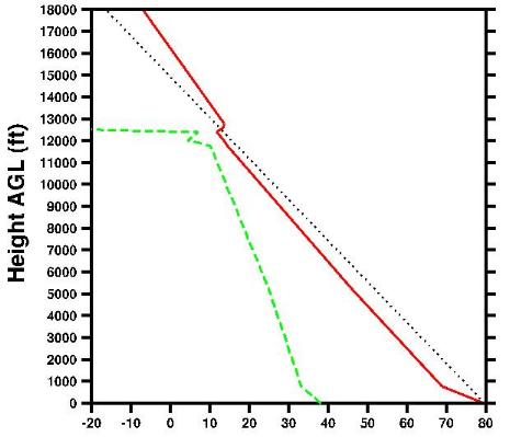
Layer. The figure gives an example of a convective Boundary
Layer (BL), from a 00Z radiosonde observation taken at Reno on a
strongly convective day. The solid red line gives the
temperature profile while the dashed green line is the dew point
temperature and the dotted black line is a DALR adiabat which begins
ar the radiosonde surface temperature. Features
distinctive of strong thermal action are: (1) the unstable
temperature lapse rate immediately above the surface, which is called
the surface layer, (2) the layer of well-mixed air above
that, called the mixed layer, which can be divided into a lower
region with a lapse rate roughly equal to the DALR up to about mid-BL
and an upper region of slightly stable lapse rate, and (3) a very
stable layer just above the top of the mixed layer, which marks the
top of the thermals and is called the "capping inversion"
(though its lapse rate is not always so stable that the temperature
actually increases with height). On weaker thermal days,
(1) the region of unstable lapse rate near the surface will be
thinner, and possibly not observable on a sounding, (2) the
temperature difference between the surface temperature and the
mixed-layer temperature will be smaller, (3) the mixed layer
will be slightly stable throughout, with no approximately DALR region,
and (4) the capping inversion will be weaker and probably not
detectable. The decrease of dew point temperature with height,
such that it approaches the temperature at the mixed-layer top, is
common in a convective boundary layer. Here the dew point is
within 4°F of the temperature line near the mixed-layer top, so
extensive cloud formation, such as is associated with
overdevelopment, is possible at that height since a difference of
4°F (2°C) is typical of cloud formation. (but note that a
larger temperature-dewpoint difference can still produce
scattered clouds). Note that the air above the
mixed layer is relatively dry and the dew point decreases dramatically
above the mixed-layer top - this often occurs, since the surface is a
source of both moisture and heat and both are carried upward by the
thermals, and can be a distinctive secondary indication of the thermal
tops.
The region of air
mixed by thermals is called the atmospheric convective Boundary
Layer. The figure gives an example of a convective Boundary
Layer (BL), from a 00Z radiosonde observation taken at Reno on a
strongly convective day. The solid red line gives the
temperature profile while the dashed green line is the dew point
temperature and the dotted black line is a DALR adiabat which begins
ar the radiosonde surface temperature. Features
distinctive of strong thermal action are: (1) the unstable
temperature lapse rate immediately above the surface, which is called
the surface layer, (2) the layer of well-mixed air above
that, called the mixed layer, which can be divided into a lower
region with a lapse rate roughly equal to the DALR up to about mid-BL
and an upper region of slightly stable lapse rate, and (3) a very
stable layer just above the top of the mixed layer, which marks the
top of the thermals and is called the "capping inversion"
(though its lapse rate is not always so stable that the temperature
actually increases with height). On weaker thermal days,
(1) the region of unstable lapse rate near the surface will be
thinner, and possibly not observable on a sounding, (2) the
temperature difference between the surface temperature and the
mixed-layer temperature will be smaller, (3) the mixed layer
will be slightly stable throughout, with no approximately DALR region,
and (4) the capping inversion will be weaker and probably not
detectable. The decrease of dew point temperature with height,
such that it approaches the temperature at the mixed-layer top, is
common in a convective boundary layer. Here the dew point is
within 4°F of the temperature line near the mixed-layer top, so
extensive cloud formation, such as is associated with
overdevelopment, is possible at that height since a difference of
4°F (2°C) is typical of cloud formation. (but note that a
larger temperature-dewpoint difference can still produce
scattered clouds). Note that the air above the
mixed layer is relatively dry and the dew point decreases dramatically
above the mixed-layer top - this often occurs, since the surface is a
source of both moisture and heat and both are carried upward by the
thermals, and can be a distinctive secondary indication of the thermal
tops.
The maximum thermalling height is expected to be somewhat lower than
the top of the mixed layer. For this case the TI=0 adiabat based
upon the surface temperature coincides, somewhat fortuitously, with the middle of the capping inversion,
so the actual mixed-layer top is associated with a TI value just slightly
below TI=0. However, with stronger (weaker) mixing the unstable layer
near the surface will be deeper (shallower) and the TI=0 adiabat will then lie to the
right (left) of the capping inversion, in which case the TI=0 height will overpredict (underpredict)
the thermalling height and a lower (higher) TI value is then associated with the
thermalling height. In general, on more strongly convective days
the thermalling height will be associated with a smaller TI value than
on weaker convective days.
(I should note that
the features described
above are more apparent in observed soundings than
in the TIP plots since the latter have coarser vertical resolution. But even observed sounding plots do not depict the exact
temperature profile in the mixed layer since not all measured
temperatures are plotted, only temperatures at "significant levels". For example, the atmospheric temperature profile in the above figure should be more rounded than the straight-line segments portray.)
Development of the Convective Boundary
Layer
To understand the TI method, and
particularly to interpret a PM plotted sounding, the user needs some
understanding of how the temperature structure close to the ground
develops with time on a typical day with convective thermals. In
the morning thermals are not present so their mixing influence is not
yet felt. Typically the AM lapse rate near the ground will be
relatively stable and unmixed, an example being the early AM sounding
shown below - but occasionally strong winds may produce an initial
mixed layer. As the sun rises and surface heating begins,
thermals develop and mix the air close to the ground, eroding the
stable layer from below to form a mixed layer with approximately a
DALR. As the heating continues the thermals grow in strength and
height, mixing more deeply. The depth of the mixed layer, or
approximately DALR region, then increases as the thermals continually
erode into the stable atmosphere above the mixing region. It is
important to recognize that mixed-layer top, i.e. the top of the
approximately DALR region, coincides with the thermal tops (since the
thermal is creating the mixing) and this is (roughly) the expected
maximum thermalling height. Generally the lapse rate in the
mixed layer is closest to the DALR sometime after noon, when the
mixing is strongest; at other times the lapse rate is slightly more
stable. In the afternoon the thermals weaken somewhat but
because a neutral stability mixed layer is already present, and thus
resistance to vertical motion is weak, they still tend to maintain the
existing mixed-layer depth. Near sunset, with a loss of surface
heating, the thermals die out and the temperature structure becomes
increasingly more stable.
PART II: SOUNDING ANALYSIS
Note: For simplicity the plots below use Temperature as
the horizontal axis and Height as the vertical axis. The same
principles can be utilized in analyzing a "SkewT" diagram in which the
Temperature axis is skewed from the horizontal and Pressure is the
vertical axis - but the SkewT plots will look, er, skewed from those
presented below.
Idealization of the Convective Boundary Layer:
the Thermal Index method
 The TI (Thermal Index) method
idealizes the convective boundary layer to estimate the mixed-layer top,
and thereby the maximum thermalling height. For an initial
morning sounding and a predicted maximum surface temperature
(Tmax), the TI method simply assumes that the afternoon
temperature profile will be a perfectly-mixed DALR layer. A DALR
adiabat line is therefore extended from the surface Tmax until it
intersects the AM sounding profile, to give the level where
TI=0. Air below that height is considered to be well mixed by
the thermals, while air above that height is considered
unaffected. Thus the TI method "predicts" how a PM temperature
profile will differ from the AM temperature profile, but it assumes
that the difference results only from thermal mixing and that the
mixing will be perfect. The maximum thermalling height is then
assumed to be at or somewhat below the TI=0 height.
The TI (Thermal Index) method
idealizes the convective boundary layer to estimate the mixed-layer top,
and thereby the maximum thermalling height. For an initial
morning sounding and a predicted maximum surface temperature
(Tmax), the TI method simply assumes that the afternoon
temperature profile will be a perfectly-mixed DALR layer. A DALR
adiabat line is therefore extended from the surface Tmax until it
intersects the AM sounding profile, to give the level where
TI=0. Air below that height is considered to be well mixed by
the thermals, while air above that height is considered
unaffected. Thus the TI method "predicts" how a PM temperature
profile will differ from the AM temperature profile, but it assumes
that the difference results only from thermal mixing and that the
mixing will be perfect. The maximum thermalling height is then
assumed to be at or somewhat below the TI=0 height.
The numerical Thermal Index at any height is the difference
between the AM sounding temperature at that height and the "predicted"
PM temperature at that height (so negative TI values are found below
the TI=0 height). Every height has a TI "trigger
temperature": when the surface temperature reaches that trigger
temperature the TI method predicts that mixing will then reach that
height, i.e. then TI=0 at that height.
The Tmax in above example
is at an elevation equal to the sounding's release elevation, i.e. the
surface is assumed to be flat. The TI method can approximate the
mixing over nearby elevated terrain by starting the DALR adiabat at
that terrain's elevation with its expected Tmax. This assumes
that the valley sounding is also applicable to the elevated terrain,
which in many cases is a reasonable approximation.
The TI method can also be used with model PM soundings to estimate
thermalling heights. However, the TI method assumes that the
sounding temperature profile represents an unmixed atmosphere,
so numerical TI values from PM model soundings are
meaningful, and hence valid, only for heights above the top of the
mixed layer predicted by the model. (Being a valid
prediction is not the same as saying that it is a correct
prediction - the latter depends upon whether the TI-assumed Tmax
is accurate!) This also implies that the TI method is
generally invalid and should not be used if the Tmax utilized for the
TI adiabat is smaller than the model-predicted Tmax, since in such
a case the adiabat from the TI-assumed Tmax will not intersect
the sounding temperature profile below the top of the mixed layer
predicted by the model (and may not intersect the temperature profile
anywhere!).
Non idealized Convective Boundary Layers:
model predicted PM soundings
While the TI method uses idealized mixing assumptions to predict PM temperature
profiles, numerical weather models predict PM temperature profiles by using
complex differential equations which include many factors besides mixing.
Starting from an AM "initialization" profile, the model marches forward
in time, calculating the temperature change at specific levels corresponding
to model grid points. The model calculations tend to produce a "well
mixed" profile when thermal mixing occurs, but just as mixing is seldom
perfect in the real atmosphere the "well mixed" profiles predicted by the
models are often not perfectly mixed. In addition, the PM model predictions
include changes occurring above the mixed layer due to effects such as
downward atmospheric motion (subsidence), effects which affect afternoon
soaring but which are omitted when one considers only the AM sounding.
Analysis of a PM model sounding plot is the best method of
estimating the maximum thermalling height for that soaring day.
Due to the variety of thermal profiles that can occur, using the
brain's pattern recognition capability to visually determine the
predicted top of the mixed layer will provide a better estimate than
any summary number that a computer can calculate. Additionally,
the human eye can judge the degree to which the atmosphere is
predicted to be truly "well mixed": if the predicted lapse rate is
noticeably less than the DALR then the thermalling can be expected to
be degraded. Cloud bases can also be estimated for
overcast or near overcast conditions (scattered clouds are difficult
to predict visually from a sounding, but are more likely
as the difference between the predicted temperature and dew point
temperature decreases). However atmospheric complexity and model
limitations can produce interpretation difficulties. For
example, estimating the top of the mixed layer can be ambiguous
when the lapse rate above the mixed layer is not very different from
the lapse rate in the mixed layer. Still, a computer summary
estimate is always more subject to error than is a knowledgeable
eyeball estimate. One caveat is that PM model soundings used in
the TIP represent conditions at 00Z, after the time of maximum
heating, and thus their surface temperature is below the day's Tmax
and their maximum thermal height tends to be somewhat
underpredicted. Also, of course, they are only model predictions
- the real atmosphere may differ!
Clouds
I need to say something about
clouds, since their effects will appear in sounding profiles, but I
will say as little as possible. Clouds form when cooling reduces
the atmospheric temperature to the dew point temperature, condensing
water vapor into liquid water. This condensation
releases heat aloft, increasing the buoyancy of the thermals and
altering the lapse rate of a perfectly mixed cloud to become the MALR [Moist Adiabatic Lapse Rate] instead of
the DALR. The MALR is always larger
than the DALR, which would be interpreted as being "stable" if the
atmosphere were dry (but it is not).
Condensation is considered likely when the difference between the
atmospheric temperature and the dew point temperature is about 4°F
(2°C). Remembering that model predictions are for
area-averages, "extensive clouds" (overcast or broken clouds)
will be indicated in a sounding when the dew-point temperature is
within 4°F of the atmospheric temperature and the temperature slope
will then be the MALR), i.e. slightly more
"stable" than the DALR. Scattered cloud conditions cannot be
adequately predicted from the TIP sounding plot, since it lacks lines
of constant humidity mixing ratio. [As an aside, if a sounding
is plotted on a SkewT diagram then the absence/existence of BL clouds
can be crudely predicted by noting whether the dew-point temperature
of the maximum humidity mixing ratio within the BL, which typically
occurs at the surface, intersects the atmospheric temperature anywhere
within the BL: if it does not then no clouds are predicted, whereas if
it does then clouds formation is predicted with the degree of sky
coverage increasing as the overlap increases.]. I should note
that moisture (and hence cloud) prediction is a notable weakness of
meteorological models, so cloud predictions should be taken with a
large grain of salt.
TI vs Model PM height prediction
The
TIP PM sounding plots actually give two predictions for the PM
temperature profile: one from the TI method, using a NWS predicted
surface temperature with an idealized mixed-layer profile, and the
other predicted by a model, using its internally computed surface
temperature and temperature profile. Which is the "best"
estimate? Life, or at least meteorology, is not simple and the
answer is "neither". I have more faith in the NWS predicted
Tmax than in the model-predicted surface temperature Tsfc, because the
former is often "tuned" to a particular location whereas the model
temperature is more generic. However, the shape of the model
temperature profile is more likely to agree with the actual
atmospheric profile than is the idealized straight line assumed by the
TI method. Therefore, I try to meld the two profiles together,
mentally shifting the model prediction such that at the lowest plotted
elevation its temperature matches the TI method temperature, and
thereby estimate the resulting top of the mixed layer, which I assume to be the
maximum thermalling height.
When the TI-predicted Tmax is
warmer than the model-predicted Tsfc, this generally
means that the expected mixed-layer top, and thus the expected maximum
thermalling height, is just below the TI=0 height. When the
TI-predicted Tmax is cooler than the model-predicted Tsfc, then
the model-predicted mixed-layer top must be decreased accordingly to
give the expected mixing height. Remeber that numerical TI values
from PM model soundings are valid only for heights above the top of
the mixed layer predicted by the model, so
the TI method should not be used if the actual surface
temperature is believed to be smaller than the
model-predicted surface temperature.
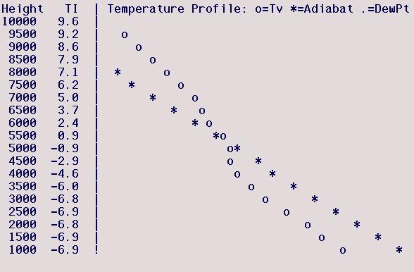
Example Interpretations
I
will evaluate several example PM MAPS model soundings as plotted in
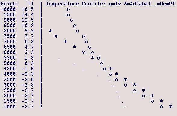
the TIP format to illustrate how such plots can be analyzed. In
these plots height is the vertical axis and temperature is the
horizontal axis. No numerical scale is given for the temperature
axis, but each column represents 1°F. Circles represent the
predicted model (virtual) temperature at 500 ft height
increments. Dots depict the predicted dew point
temperature. The plots also include the TI-method estimate of
the PM temperature profile plotted as asterisks, i.e. a DALR adiabat
extending from the surface Tmax predicted by the NWS
(not by the model). The slope of the adiabat indicates the
(approximate) slope expected for any mixed layer in the
sounding. And finally, note that the limited resolution of the
plots and of the models means that details of the mixed layer are
often smoothed out; observed soundings have higher resolution and the
features described in the "Convective Boundary Layer" section above
are more apparent in those soundings than in the present plots (but
even observed sounding plots do not depict the exact temperature
profile in the mixed layer since they do not plot all measured
temperatures but only temperatures at "significant levels") Note
that the model predicts its own surface temperature, which I will call
Tsfc, which may differ from the Tmax assumed for the TI-method
adiabat. Also note that the plots only extend down to 500 ft and
therefore omit the surface itself. And finally, note that the
limited resolution of the plots and of the models means that details
of the mixed layer are often smoothed out so predictions of the
maximum thermalling height have a "fuzziness" of around 500 ft.
Avenal (Lemoore), Jan 30, 2001
This case is similar to the strongly
convective boundary layer illustrated above. The model lapse rate is
well-mixed, essentially a DALR, up to 3500 ft. The
model-predicted top of the mixed layer is best determined by noting that the
region above the DALR region has an essentially constant lapse rate
that intersects with the DALR region around 4000 ft. The dew
point drops dramatically above 3500 ft, suggesting a mixing height
between 3500-4000 ft. So the best estimate of the
model-predicted maximum thermalling height is between 3500-4000
ft. The dew point is very close to the atmospheric temperature
at 3500 ft, indicating that thin clouds may form at the top of the
mixed layer. The model-predicted Tsfc is slightly lower than
the TI-assumed Tmax (a NWS prediction), by
about 3°F (3 columns). The warmer TI-assumed Tmax predicts a
somewhat higher mixed-layer top of 4750 ft, which is the
TI=0 height - note this is above the model-predicted mixed-layer top and is therefore a meaningful TI prediction for the
TI-assumed Tmax . Melding the two predictions together, and
relying on the TI-method's NWS Tmax to be a more accurate surface
temperature prediction, I would estimate the maximum thermalling
height to be around 4250 ft.
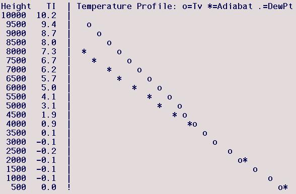
Avenal (Lemoore), Mar 28, 2001
The model predicts a nearly DALR
(actually very slightly stable) mixed layer extending to a height of
around 3000 ft, above which the stability increases somewhat
before becoming very stable between 4500 and 5000 ft. The latter
marks the capping inversion, so the top of the model's mixed layer is
around 4500 ft. Note that the model's Tsfc is significantly
lower than the TI-assumed Tmax, which predicts a mixed-layer top
(TI=0) of 5250 ft (meaningful because it is above the
model-predicted mixed-layer top). Melding the two
predictions together, and placing more weight on the TI-assumed Tmax,
I would estimate a maximum soaring height of around 5000 ft.
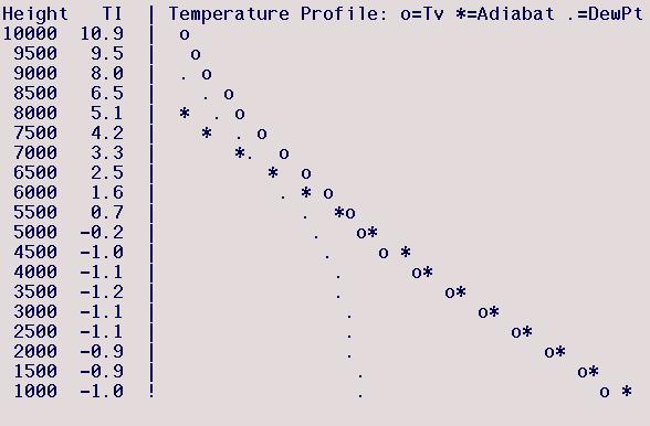
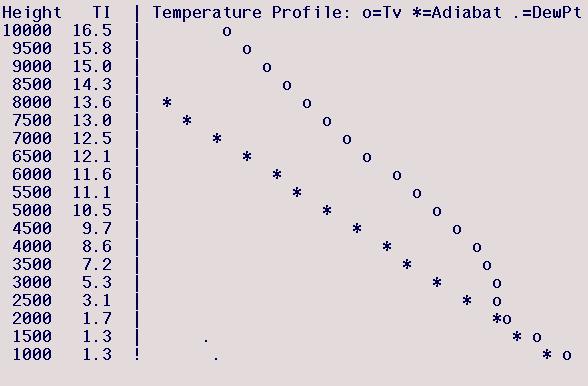
Williams (Marysville), Mar 27, 2001
The PM model sounding has a nearly
DALR mixed layer up to a height of 4000 ft. The lapse rate
becomes slightly stable up to 4500 ft, then a more strongly stable
region exists between 4500-5000 ft, above which there is a deep layer
of slight stability. Determining the top of the model's
mixed-layer In cases such as this where the lapse rate above the
mixed layer does not differ markedly from the lapse rate in the upper
mixed layer can be difficult, but here the more stable layer seems to
be a capping inversion so I estimate the top of the model-predicted
mixed layer to be 4500 ft. Here the model-predicted Tsfc and
TI-assumed Tmax are very close. There are actually two TI=0
heights, at 900 and 3500 ft (see the TI column since the circles
overplot the asterisk) but neither are meaningful since they are
below the model-predicted mixed-layer top, and thus are
not meaningful predictions. So the estimated thermalling
height is the model's mixed-layer top, 4500 ft.
Avenal (Lemoore), Feb 10, 2001
Just above the surface the
model-predicted lapse rate is nearly DALR up to 4500 ft, above which
it is moderately "stable". However, 5000 ft appears to be a
cloud base since the dew point there nears the atmospheric temperature
and nearly parallels it above that - so thermals likely extend
above 5000 ft and the "stable" lapse rate there is really the
adiabatic lapse rate (MALR). Here
the maximum soaring height will be below 5000 ft due to the cloud
base.
Hollister (Oakland), Mar 22, 2001
The model predicts a shallow
mixed layer up to 1000 ft, above which is a strongly stable inversion
layer. The TI-assumed Tmax is much larger than the
model-predicted Tsfc. This forecast is for Hollister so I
greatly favor the NWS Tmax predictions, since the model Tsfc
predictions are for an Oakland location, and would predict the top of
the mixed layer to occur at the TI=0 height between 2000-2500
ft. Note that TI =0 height is above the model-predicted mixed-layer
top and is thus meaningful.
Avenal (Lemoore), Feb 6, 2001
The model-predicted well-mixed DALR
layer extends to 2000 ft, above which the sounding is strongly stable,
so the model's mixed-layer top is between 2000-2500 ft. Note
that the TI adiabat never intersects the model-predicted temperature
profile so there is officially no TI=0 height - this occurs
because the TI-assumed surface temperature is cooler than the
model-predicted surface temperature in which case use of the TI method
is generally invalid, as occurs here. One's eyeball indicates
that the model-predicted temperature profile is just slightly warmer
than the the TI-predicted adiabat so the model-predicted mixed-layer
temperature is essentially correct and its mixed-layer top is also
essentially correct, though slightly greater than would be predicted
if the model Tmax equalled the NWS predicted Tmax. Weighting the
NWS Tmax more heavily here means that the expected thermalling height
will be slightly below the model-predicted mixed-layer top, and I
would estimate it to be 2000 ft.
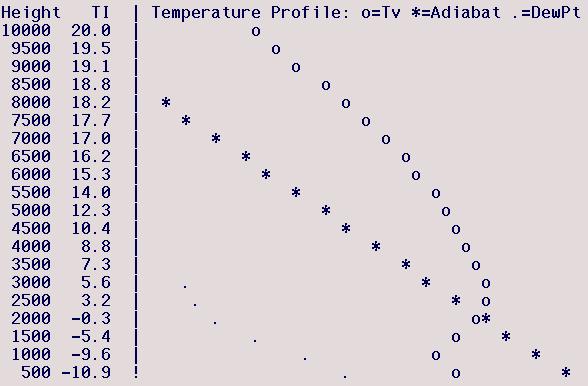
Williams (Marysville), Jan 31, 2001
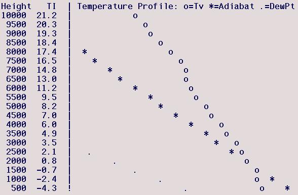
Here the model-predicted profile has
no well-mixed layer. The model's lapse rate between 500-1000 ft
is moderately stable, with a very stable region between 1000-1500
ft. The latter may or may not be a capping inversion, but would
indicate a mixed-layer top of 1000 ft. In any event, since
the layer below that is not well-mixed any thermals are predicted to
be weak. The TI-assumed Tmax is significantly larger than the
model-predicted Tsfc and predicts a TI=0 mixed-layer top of 1750
ft. This is a meaningful prediction because this height is above
the model-predicted mixed-layer top, so I would meld the two profiles
together, weighting the TI-assumed Tmax more heavily, to predict a
maximum thermallling height of 1500 ft. But the model's
prediction of very weak thermals indicates the thermalling will be
even worse than the low mixed-layer top would indicate. This is
definitely not a day to expect to do any thermalling!
Return to the top of this page
Link to
Hollister TIP description page
Link to TIP user's experiences, to learn how other pilots use the TIP
Link to the latest TIP Forecasts, a listing of all TIP sites, and TIP email subscription information
Link to
DrJack's home page